Easy does it

Published: 2017-06-15

SUMMARY: An example of the amazing concision of the R language is provided. Also: functions as objects; plotting.

I recently needed a structure representing points randomly distributed in an n-dimensional space. A natural way to represent such points is a matrix, with each row corresponding to a point and with the n columns of the matrix corresponding to the n coordinates of the space.

I was delighted to find that I could generate such a matrix, in the R language, with a single line of code. In the code shown below I have wrapped the single line of code in a function. As you can see, the body of the function, not counting comments, is one line.

gen_points = function(dim=2, num=10, FUN=rnorm) {
  #dim: The dimension of the space in which the points reside.
  #num: The number of points.
  #FUN: The random function used to generate coordinate values.
  matrix(FUN(dim * num), nrow=num)
}
	

The trick is to provide the matrix function with a vector of length dimension * number of points. You also tell the matrix function how many rows, or columns, the matrix should have—either one will do.

Cycling through functions

Another convenient feature of R is that functions can be passed around like any other object. This is shown in the gen_points function defined above, where the third argument of gen_points is an arbitrary function taking one argument. Let's demonstrate how convenient this is by generating a few plots using different random functions.

source('gen_points.r')

gen_plots = function() {
  num = 2^12 #Number of points in each plot.
  height = width = 750 #Image dimensions in pixels.
  #A list of random functions.
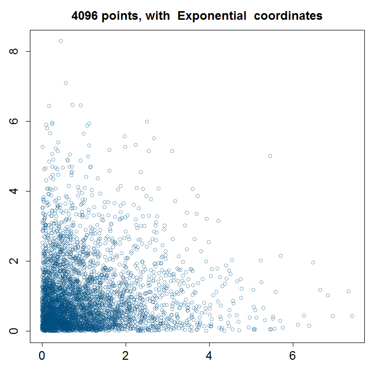
  functions = c(rexp, runif, rnorm, rcauchy)
  names = c('Exponential', 'Uniform', 'Normal', 'Cauchy')
  #Make sure each function has a name.
  stopifnot(length(functions) == length(names))

  #For each function generate a plot.
  for (ii in 1:length(functions)) {
    filename = paste(names[ii], '.png', sep='')
    png(filename=filename, height=height, width=width)
    #functions is a list; therefore, each element must be accessed with double brackets.
    mat = gen_points(2, num, functions[[ii]])
    main = paste(num, 'points, with ', names[ii], ' coordinates')
    plot(mat, main=main, cex.main=2, cex.axis=2, mgp=c(0, 1.5, 0),
      col=rgb(0, 0.3, 0.5, 1/2), cex=1.5, xlab='', ylab='')
    dev.off()
  }
}
	

In addition to the matrix of data points (mat), the plot function takes additional arguments in the foregoing code:

• main=main  specify the main title
• cex.main=2  specify the font size of the main title
• cex.axis=2  specify the size of the axis tick mark labels
• mgp=c(0, 1.5, 0)  specify the space between tick marks and tick mark labels
• col=rgb(0, 0.3, 0.5, 1/2)  set the color and transparency (1/2) of the plot points

  When a plot contains many points it is helpful to make the points partially transparent. This way, in areas where many points overlap there is a darkening that signals a high density of points.

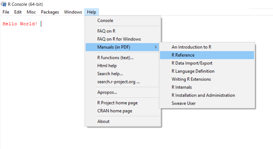
• cex=1.5  increase the size of the plot points from their default by 50%
• xlab='', ylab=''  eliminate axis titles

plot can take many additional arguments. See the chapter on "The graphics package" in the R Reference Manual that comes with every installation of R. You can access the R Reference Manual from the R Console menu:

The plots that are generated by the gen_plots function are as follows:

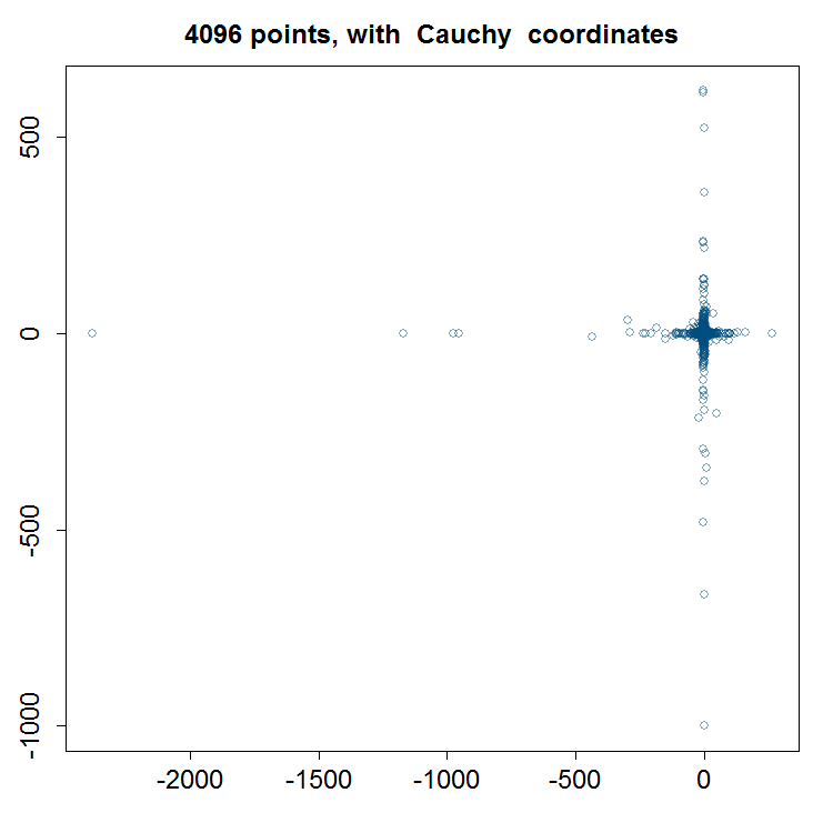
The Cauchy plot tends to be cross shaped. This is because the Cauchy distribution has fat tails, meaning it is prone to generate extreme values. However, it is rare for two extreme values to be generated at the same time (assuming the x and y coordinates are statistically independent). Therefore, we get a plot where extreme x values tend to be paired with moderate y values, and extreme y values tend to be paired with moderate x values. This generates the cross shaped plot that we observe.